Dotplot for model coefficients
coefplot.RdA graphical display of the coefficients and standard errors from a fitted model
coefplot is the S3 generic method for plotting the coefficients from a fitted model.
This can be extended with new methods for other types of models not currently available.
Dotplot for coefficients
Usage
coefplot(model, ...)

# S3 method for default
coefplot(
  model,
  title = "Coefficient Plot",
  xlab = "Value",
  ylab = "Coefficient",
  innerCI = 1,
  outerCI = 2,
  innerType = 1,
  outerType = 1,
  lwdInner = 1 + interactive * 2,
  lwdOuter = if (interactive) 1 else unname((Sys.info()["sysname"] != "Windows") * 0.5),
  pointSize = 3 + interactive * 5,
  color = "blue",
  shape = 16,
  cex = 0.8,
  textAngle = 0,
  numberAngle = 0,
  zeroColor = "grey",
  zeroLWD = 1,
  zeroType = 2,
  facet = FALSE,
  scales = "free",
  sort = c("natural", "magnitude", "alphabetical"),
  decreasing = FALSE,
  numeric = FALSE,
  fillColor = "grey",
  alpha = 1/2,
  horizontal = FALSE,
  factors = NULL,
  only = NULL,
  shorten = TRUE,
  intercept = TRUE,
  interceptName = "(Intercept)",
  coefficients = NULL,
  predictors = NULL,
  strict = FALSE,
  trans = identity,
  interactive = FALSE,
  newNames = NULL,
  plot = TRUE,
  ...
)

# S3 method for data.frame
coefplot(
  model,
  title = "Coefficient Plot",
  xlab = "Value",
  ylab = "Coefficient",
  interactive = FALSE,
  lwdInner = 1 + interactive * 2,
  lwdOuter = if (interactive) 1 else unname((Sys.info()["sysname"] != "Windows") * 0.5),
  pointSize = 3 + interactive * 5,
  color = "blue",
  cex = 0.8,
  textAngle = 0,
  numberAngle = 0,
  shape = 16,
  innerType = 1,
  outerType = 1,
  outerCI = 2,
  innerCI = 1,
  multi = FALSE,
  zeroColor = "grey",
  zeroLWD = 1,
  zeroType = 2,
  numeric = FALSE,
  fillColor = "grey",
  alpha = 1/2,
  horizontal = FALSE,
  facet = FALSE,
  scales = "free",
  value = "Value",
  coefficient = "Coefficient",
  errorHeight = 0,
  dodgeHeight = 1,
  ...
)

# S3 method for lm
coefplot(...)

# S3 method for glm
coefplot(...)

# S3 method for workflow
coefplot(model, ...)

# S3 method for model_fit
coefplot(model, ...)

# S3 method for rxGlm
coefplot(...)

# S3 method for rxLinMod
coefplot(...)

# S3 method for rxLogit
coefplot(...)
Arguments
- model
A data.frame like that built from coefplot(..., plot=FALSE)
- ...
Further Arguments
- title
The name of the plot, if NULL then no name is given
- xlab
The x label
- ylab
The y label
- innerCI
How wide the inner confidence interval should be, normally 1 standard deviation. If 0, then there will be no inner confidence interval.
- outerCI
How wide the outer confidence interval should be, normally 2 standard deviations. If 0, then there will be no outer confidence interval.
- innerType
The type of the inner CI line, 0 will mean no line
- outerType
The type of the outer CI line, 0 will mean no line
- lwdInner
The thickness of the inner confidence interval
- lwdOuter
The thickness of the outer confidence interval
- pointSize
Size of coefficient point
- color
The color of the points and lines
- shape
The shape of the points
- cex
The text size multiplier, currently not used
- textAngle
The angle for the coefficient labels, 0 is horizontal
- numberAngle
The angle for the value labels, 0 is horizontal
- zeroColor
The color of the line indicating 0
- zeroLWD
The thickness of the 0 line
- zeroType
The type of 0 line, 0 will mean no line
- facet
logical; If the coefficients should be faceted by the variables, numeric coefficients (including the intercept) will be one facet
- scales
The way the axes should be treated in a faceted plot. Can be c("fixed", "free", "free_x", "free_y")
- sort
Determines the sort order of the coefficients. Possible values are c("natural", "magnitude", "alphabetical")
- decreasing
logical; Whether the coefficients should be ascending or descending
- numeric
logical; If true and factors has exactly one value, then it is displayed in a horizontal graph with continuous confidence bounds.
- fillColor
The color of the confidence bounds for a numeric factor
- alpha
The transparency level of the numeric factor's confidence bound
- horizontal
logical; If the plot should be displayed horizontally
- factors
Vector of factor variables that will be the only ones shown
- only
logical; If factors has a value this determines how interactions are treated. True means just that variable will be shown and not its interactions. False means interactions will be included. Currently not available.
- shorten
logical or character; If
FALSEthen coefficients for factor levels will include their variable name. IfTRUEcoefficients for factor levels will be stripped of their variable names. If a character vector of variables only coefficients for factor levels associated with those variables will the variable names stripped. Currently not available.- intercept
logical; Whether the Intercept coefficient should be plotted
- interceptName
Specifies name of intercept it case it is not the default of "(Intercept"). Currently not available.
- coefficients
A character vector specifying which factor coefficients to keep. It will keep all levels and any interactions, even if those are not listed.
- predictors
A character vector specifying which coefficients to keep. Each individual coefficient can be specified. Use predictors to specify entire factors.
- strict
If TRUE then predictors will only be matched to its own coefficients, not its interactions
- trans
A transformation function to apply to the values and confidence intervals.
identityby default. Useinvlogitfor binary regression.- interactive
If `TRUE` an interactive plot is generated instead of `[ggplot2]`
- newNames
Named character vector of new names for coefficients
- plot
logical; If the plot should be drawn, if false then a data.frame of the values will be returned
- multi
logical; If this is for
multiplotthen leave the colors as determined by the legend, if FALSE then make all colors the same- value
Name of variable for value metric
- coefficient
Name of variable for coefficient names
- errorHeight
Height of error bars
- dodgeHeight
Amount of vertical dodging
Value
A ggplot2 object or data.frame. See details in coefplot.lm for more information
If plot is TRUE then a ggplot object is returned. Otherwise a data.frame listing coefficients and confidence bands is returned.
a ggplot graph object
Details
A graphical display of the coefficients and standard errors from a fitted model, this function uses a data.frame as the input.
Examples
data(diamonds)
head(diamonds)
#> # A tibble: 6 × 10
#> carat cut color clarity depth table price x y z
#> <dbl> <ord> <ord> <ord> <dbl> <dbl> <int> <dbl> <dbl> <dbl>
#> 1 0.23 Ideal E SI2 61.5 55 326 3.95 3.98 2.43
#> 2 0.21 Premium E SI1 59.8 61 326 3.89 3.84 2.31
#> 3 0.23 Good E VS1 56.9 65 327 4.05 4.07 2.31
#> 4 0.29 Premium I VS2 62.4 58 334 4.2 4.23 2.63
#> 5 0.31 Good J SI2 63.3 58 335 4.34 4.35 2.75
#> 6 0.24 Very Good J VVS2 62.8 57 336 3.94 3.96 2.48
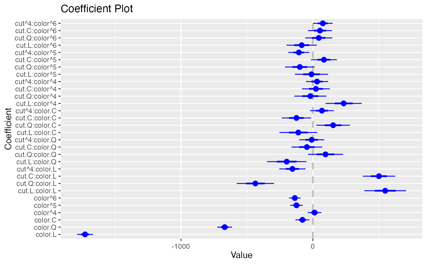
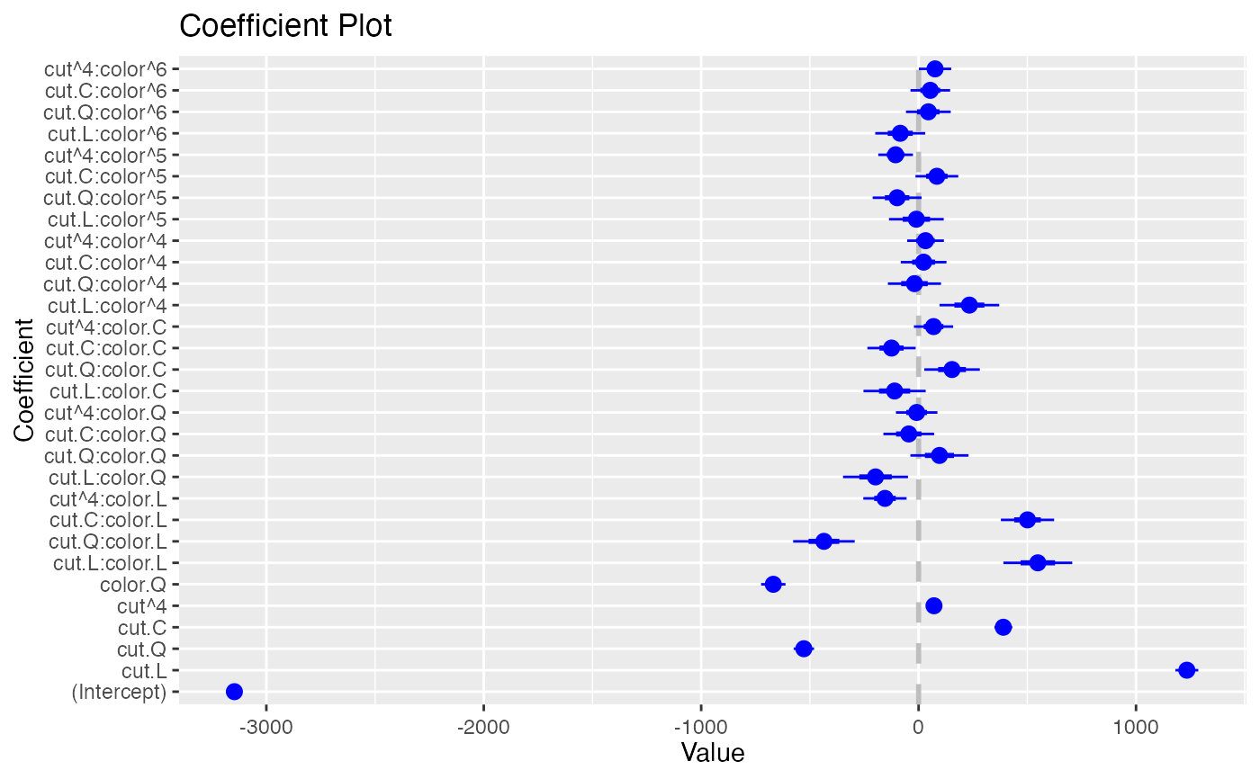
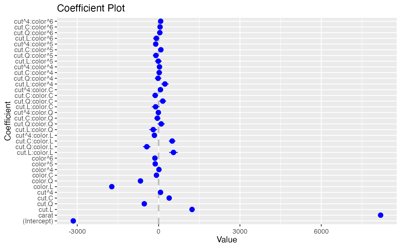
model1 <- lm(price ~ carat + cut*color, data=diamonds)
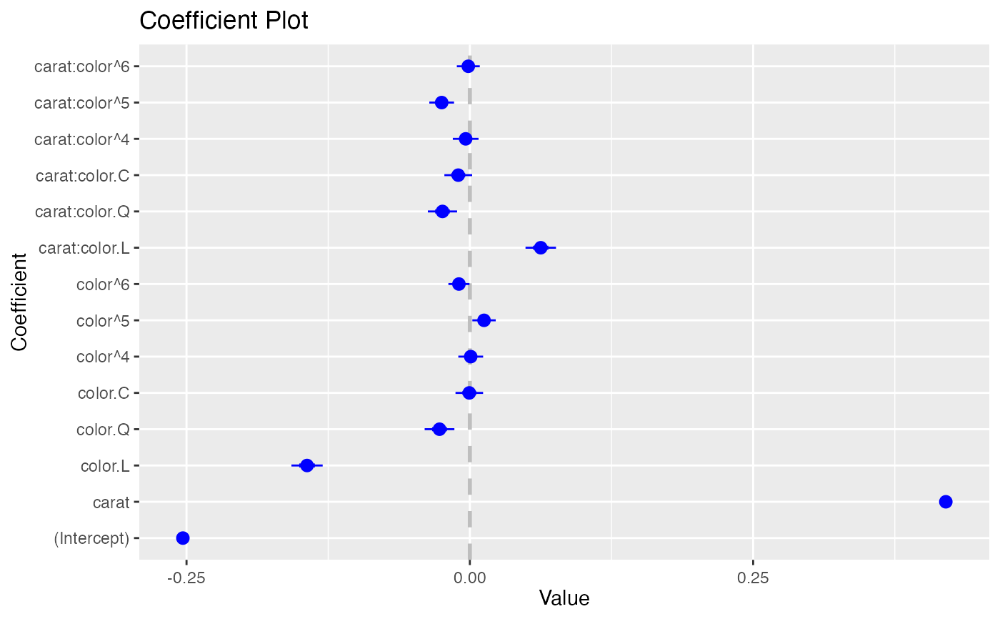
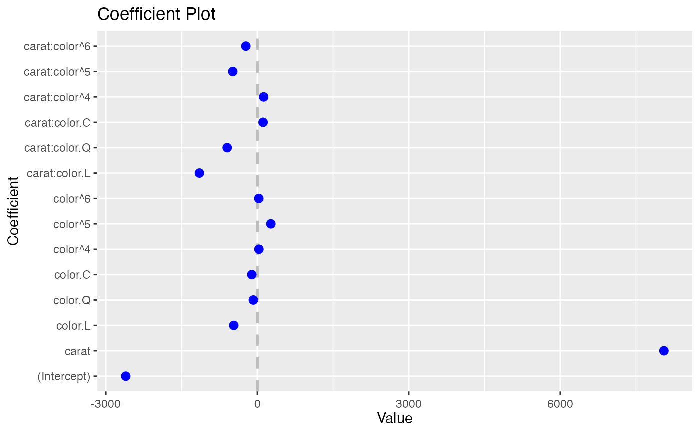
model2 <- lm(price ~ carat*color, data=diamonds)
model3 <- glm(price > 10000 ~ carat*color, data=diamonds)
coefplot(model1)
 coefplot(model2)
 coefplot(model3)
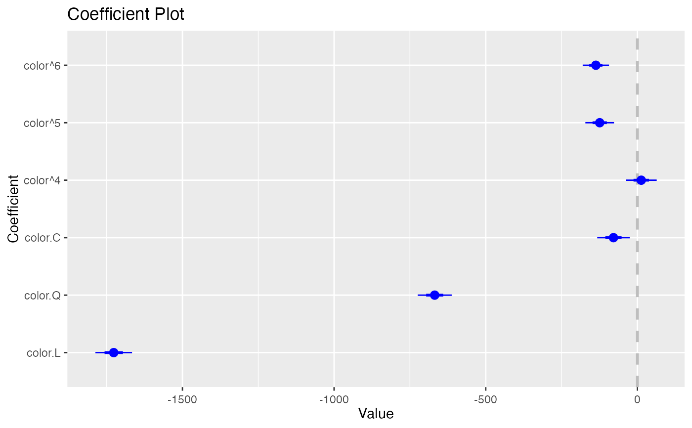
 coefplot(model1, predictors="color")
 coefplot(model1, predictors="color", strict=TRUE)
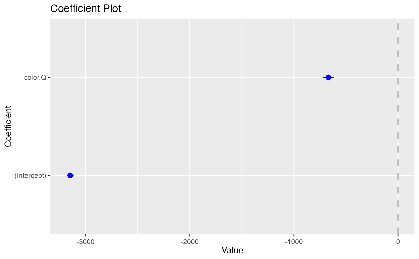
 coefplot(model1, coefficients=c("(Intercept)", "color.Q"))
 coefplot(model1, predictors="cut", coefficients=c("(Intercept)", "color.Q"), strict=TRUE)
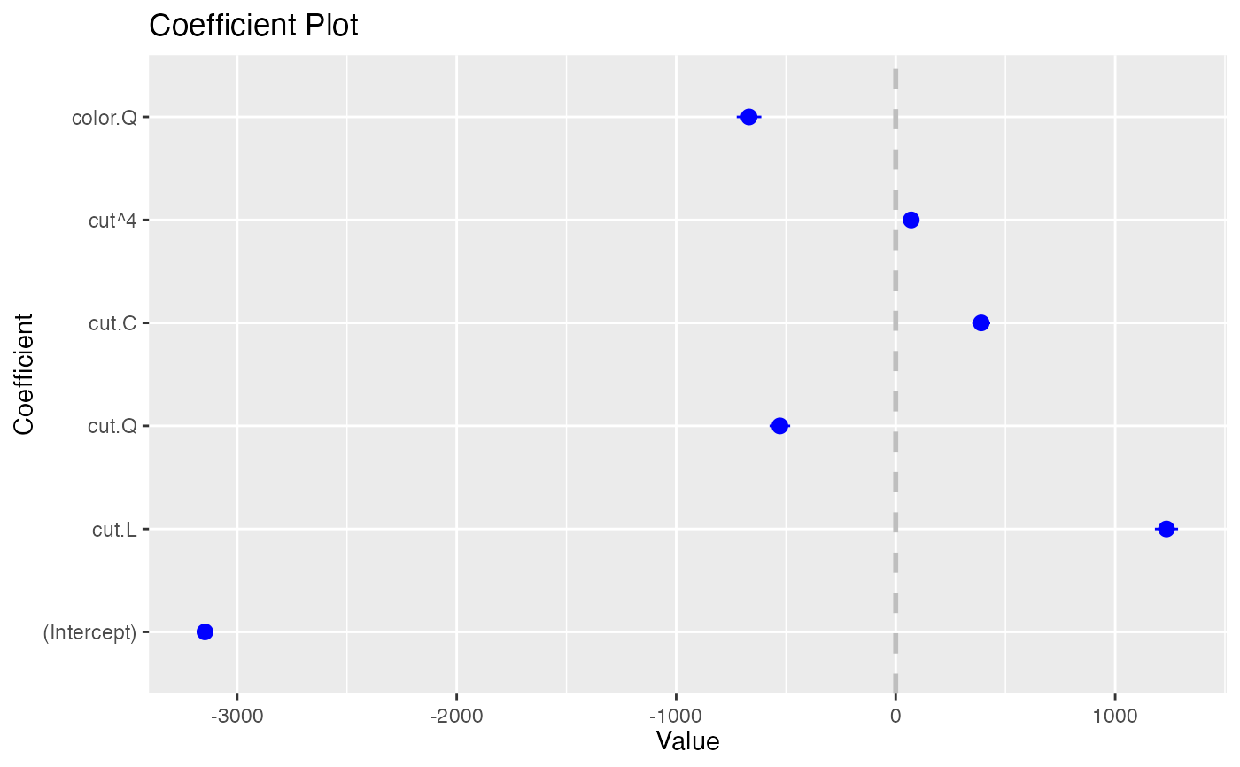 coefplot(model1, predictors="cut", coefficients=c("(Intercept)", "color.Q"), strict=FALSE)
 coefplot(model1, predictors="cut", coefficients=c("(Intercept)", "color.Q"),
strict=TRUE, newNames=c(color.Q="Color", "cut^4"="Fourth"))
coefplot(model1, predictors="cut", coefficients=c("(Intercept)", "color.Q"),
strict=TRUE, newNames=c(color.Q="Color", "cut^4"="Fourth"))
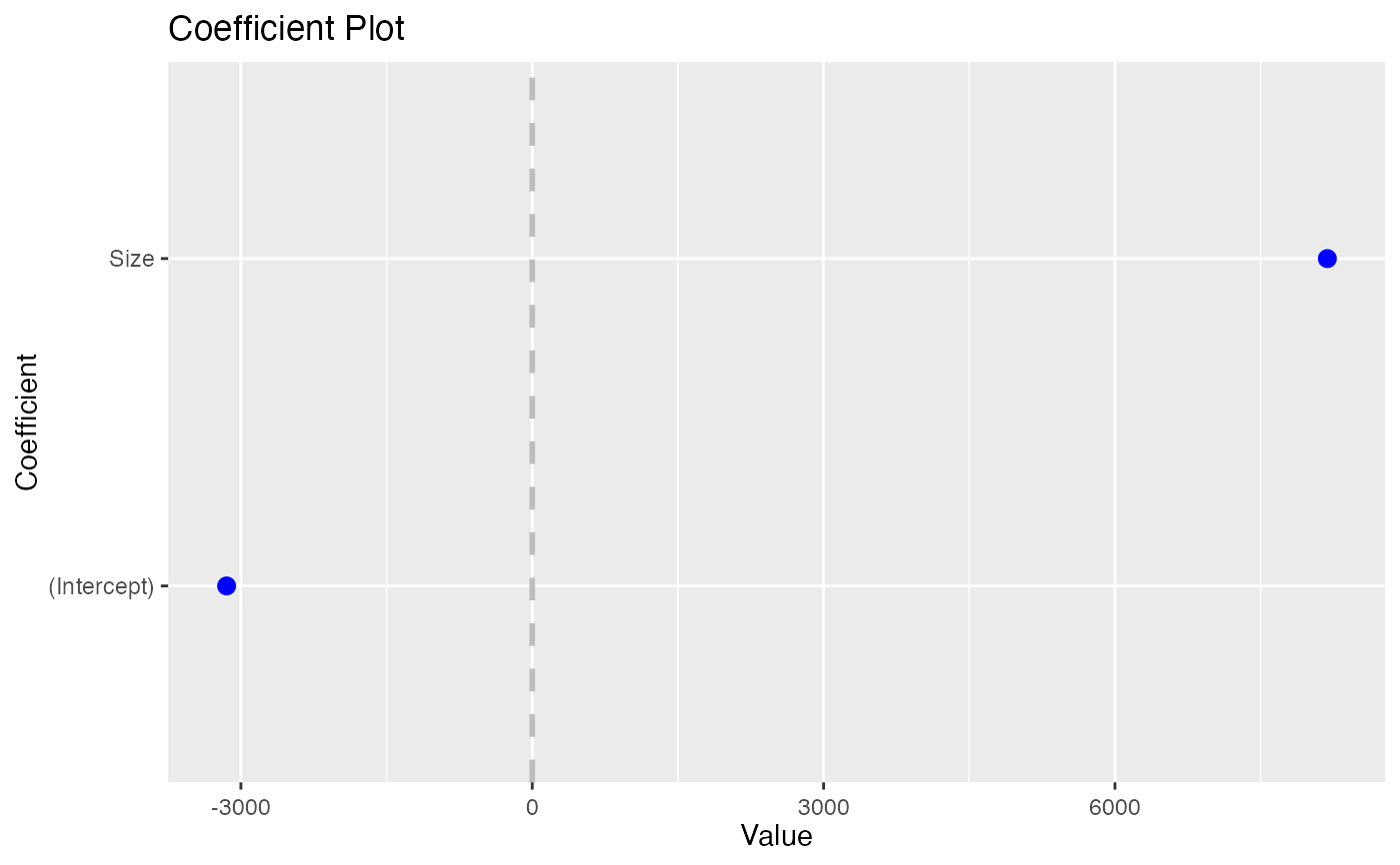
 coefplot(model1, predictors=c("(Intercept)", "carat"), newNames=c(carat="Size"))
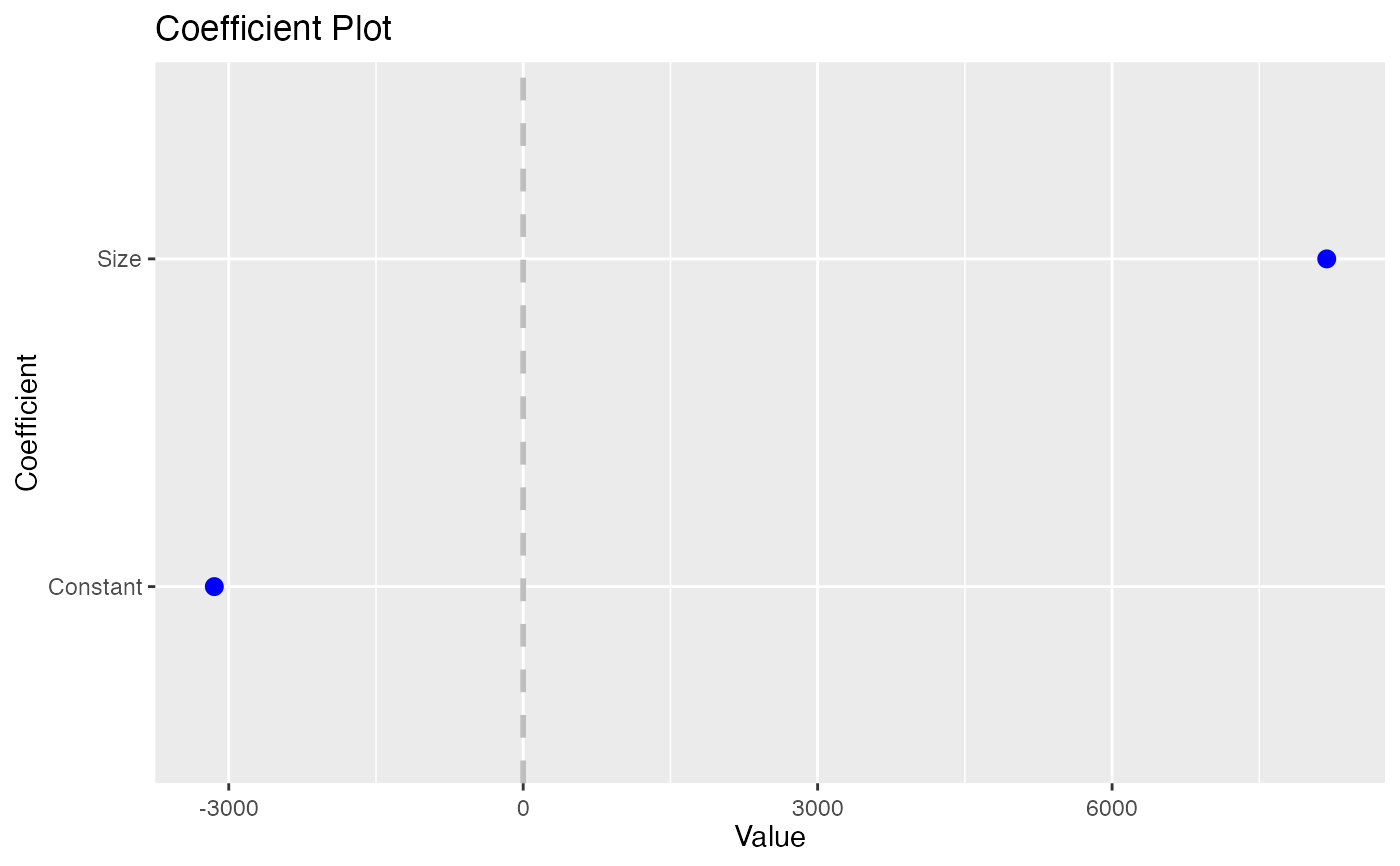
 coefplot(model1, predictors=c("(Intercept)", "carat"),
newNames=c(carat="Size", "(Intercept)"="Constant"))
coefplot(model1, predictors=c("(Intercept)", "carat"),
newNames=c(carat="Size", "(Intercept)"="Constant"))
 data(diamonds)
head(diamonds)
#> # A tibble: 6 × 10
#> carat cut color clarity depth table price x y z
#> <dbl> <ord> <ord> <ord> <dbl> <dbl> <int> <dbl> <dbl> <dbl>
#> 1 0.23 Ideal E SI2 61.5 55 326 3.95 3.98 2.43
#> 2 0.21 Premium E SI1 59.8 61 326 3.89 3.84 2.31
#> 3 0.23 Good E VS1 56.9 65 327 4.05 4.07 2.31
#> 4 0.29 Premium I VS2 62.4 58 334 4.2 4.23 2.63
#> 5 0.31 Good J SI2 63.3 58 335 4.34 4.35 2.75
#> 6 0.24 Very Good J VVS2 62.8 57 336 3.94 3.96 2.48
model1 <- lm(price ~ carat + cut*color, data=diamonds)
model2 <- lm(price ~ carat*color, data=diamonds)
coefplot(model1)
data(diamonds)
head(diamonds)
#> # A tibble: 6 × 10
#> carat cut color clarity depth table price x y z
#> <dbl> <ord> <ord> <ord> <dbl> <dbl> <int> <dbl> <dbl> <dbl>
#> 1 0.23 Ideal E SI2 61.5 55 326 3.95 3.98 2.43
#> 2 0.21 Premium E SI1 59.8 61 326 3.89 3.84 2.31
#> 3 0.23 Good E VS1 56.9 65 327 4.05 4.07 2.31
#> 4 0.29 Premium I VS2 62.4 58 334 4.2 4.23 2.63
#> 5 0.31 Good J SI2 63.3 58 335 4.34 4.35 2.75
#> 6 0.24 Very Good J VVS2 62.8 57 336 3.94 3.96 2.48
model1 <- lm(price ~ carat + cut*color, data=diamonds)
model2 <- lm(price ~ carat*color, data=diamonds)
coefplot(model1)
 coefplot(model2)
 coefplot(model1, predictors="color")
 coefplot(model1, predictors="color", strict=TRUE)
 coefplot(model1, coefficients=c("(Intercept)", "color.Q"))
 data(diamonds)
head(diamonds)
#> # A tibble: 6 × 10
#> carat cut color clarity depth table price x y z
#> <dbl> <ord> <ord> <ord> <dbl> <dbl> <int> <dbl> <dbl> <dbl>
#> 1 0.23 Ideal E SI2 61.5 55 326 3.95 3.98 2.43
#> 2 0.21 Premium E SI1 59.8 61 326 3.89 3.84 2.31
#> 3 0.23 Good E VS1 56.9 65 327 4.05 4.07 2.31
#> 4 0.29 Premium I VS2 62.4 58 334 4.2 4.23 2.63
#> 5 0.31 Good J SI2 63.3 58 335 4.34 4.35 2.75
#> 6 0.24 Very Good J VVS2 62.8 57 336 3.94 3.96 2.48
model1 <- lm(price ~ carat + cut*color, data=diamonds)
model2 <- lm(price ~ carat*color, data=diamonds)
df1 <- coefplot(model1, plot=FALSE)
df2 <- coefplot(model2, plot=FALSE)
coefplot(df1)
data(diamonds)
head(diamonds)
#> # A tibble: 6 × 10
#> carat cut color clarity depth table price x y z
#> <dbl> <ord> <ord> <ord> <dbl> <dbl> <int> <dbl> <dbl> <dbl>
#> 1 0.23 Ideal E SI2 61.5 55 326 3.95 3.98 2.43
#> 2 0.21 Premium E SI1 59.8 61 326 3.89 3.84 2.31
#> 3 0.23 Good E VS1 56.9 65 327 4.05 4.07 2.31
#> 4 0.29 Premium I VS2 62.4 58 334 4.2 4.23 2.63
#> 5 0.31 Good J SI2 63.3 58 335 4.34 4.35 2.75
#> 6 0.24 Very Good J VVS2 62.8 57 336 3.94 3.96 2.48
model1 <- lm(price ~ carat + cut*color, data=diamonds)
model2 <- lm(price ~ carat*color, data=diamonds)
df1 <- coefplot(model1, plot=FALSE)
df2 <- coefplot(model2, plot=FALSE)
coefplot(df1)
 coefplot(df2)
 if (FALSE) {
data(diamonds)
mod3 <- rxLinMod(price ~ carat + cut + x, data=diamonds)
coefplot(mod3)
}
if (FALSE) {
data(diamonds)
mod6 <- rxLogit(price > 10000 ~ carat + cut + x, data=diamonds)
coefplot(mod6)
}
if (FALSE) {
data(diamonds)
mod3 <- rxLinMod(price ~ carat + cut + x, data=diamonds)
coefplot(mod3)
}
if (FALSE) {
data(diamonds)
mod6 <- rxLogit(price > 10000 ~ carat + cut + x, data=diamonds)
coefplot(mod6)
}