Plot multiple coefplots

Plot the coefficients from multiple models

Usage

multiplot(
  ...,
  title = "Coefficient Plot",
  xlab = "Value",
  ylab = "Coefficient",
  innerCI = 1,
  outerCI = 2,
  lwdInner = 1,
  lwdOuter = (Sys.info()["sysname"] != "Windows") * 0.5,
  pointSize = 3,
  dodgeHeight = 1,
  color = "blue",
  shape = 16,
  linetype = 1,
  cex = 0.8,
  textAngle = 0,
  numberAngle = 90,
  zeroColor = "grey",
  zeroLWD = 1,
  zeroType = 2,
  single = TRUE,
  scales = "fixed",
  ncol = length(unique(modelCI$Model)),
  sort = c("natural", "normal", "magnitude", "size", "alphabetical"),
  decreasing = FALSE,
  names = NULL,
  numeric = FALSE,
  fillColor = "grey",
  alpha = 1/2,
  horizontal = FALSE,
  factors = NULL,
  only = NULL,
  shorten = TRUE,
  intercept = TRUE,
  interceptName = "(Intercept)",
  coefficients = NULL,
  predictors = NULL,
  strict = FALSE,
  newNames = NULL,
  plot = TRUE,
  drop = FALSE,
  by = c("Coefficient", "Model"),
  plot.shapes = FALSE,
  plot.linetypes = FALSE,
  legend.position = c("bottom", "right", "left", "top", "none"),
  secret.weapon = FALSE,
  legend.reverse = FALSE,
  trans = identity
)

Arguments

...: Models to be plotted
title: The name of the plot, if NULL then no name is given
xlab: The x label
ylab: The y label
innerCI: How wide the inner confidence interval should be, normally 1 standard deviation. If 0, then there will be no inner confidence interval.
outerCI: How wide the outer confidence interval should be, normally 2 standard deviations. If 0, then there will be no outer confidence interval.
lwdInner: The thickness of the inner confidence interval
lwdOuter: The thickness of the outer confidence interval
pointSize: Size of coefficient point
dodgeHeight: Amount of vertical dodging
color: The color of the points and lines
shape: The shape of the points
linetype: The type of line drawn for the standard errors
cex: The text size multiplier, currently not used
textAngle: The angle for the coefficient labels, 0 is horizontal
numberAngle: The angle for the value labels, 0 is horizontal
zeroColor: The color of the line indicating 0
zeroLWD: The thickness of the 0 line
zeroType: The type of 0 line, 0 will mean no line
single: logical; If TRUE there will be one plot with the points and bars stacked, otherwise the models will be displayed in separate facets
scales: The way the axes should be treated in a faceted plot. Can be c("fixed", "free", "free_x", "free_y")
ncol: The number of columns that the models should be plotted in
sort: Determines the sort order of the coefficients. Possible values are c("natural", "magnitude", "alphabetical")
decreasing: logical; Whether the coefficients should be ascending or descending
names: Names for models, if NULL then they will be named after their inputs
numeric: logical; If true and factors has exactly one value, then it is displayed in a horizontal graph with continuous confidence bounds.
fillColor: The color of the confidence bounds for a numeric factor
alpha: The transparency level of the numeric factor's confidence bound
horizontal: logical; If the plot should be displayed horizontally
factors: Vector of factor variables that will be the only ones shown
only: logical; If factors has a value this determines how interactions are treated. True means just that variable will be shown and not its interactions. False means interactions will be included.
shorten: logical or character; If FALSE then coefficients for factor levels will include their variable name. If TRUE coefficients for factor levels will be stripped of their variable names. If a character vector of variables only coefficients for factor levels associated with those variables will the variable names stripped.
intercept: logical; Whether the Intercept coefficient should be plotted
interceptName: Specifies name of intercept it case it is not the default of "(Intercept").
coefficients: A character vector specifying which factor coefficients to keep. It will keep all levels and any interactions, even if those are not listed.
predictors: A character vector specifying which coefficients to keep. Each individual coefficient can be specified. Use predictors to specify entire factors
strict: If TRUE then predictors will only be matched to its own coefficients, not its interactions
newNames: Named character vector of new names for coefficients
plot: logical; If the plot should be drawn, if false then a data.frame of the values will be returned
drop: logical; if TRUE then models without valid coefficients to show will not be plotted
by: If "Coefficient" then a normal multiplot is plotted, if "Model" then the coefficients are plotted along the axis with one for each model. If plotting by model only one coefficient at a time can be selected. This is called the secret weapon by Andy Gelman.
plot.shapes: If TRUE points will have different shapes for different models
plot.linetypes: If TRUE lines will have different shapes for different models
legend.position: position of legend, one of "left", "right", "bottom", "top", "none"
secret.weapon: If this is TRUE and exactly one coefficient is listed in coefficients then Andy Gelman's secret weapon is plotted.
legend.reverse: Setting to reverse the legend in a multiplot so that it matches the order they are drawn in the plot
trans: A transformation function to apply to the values and confidence intervals. identity by default. Use invlogit for binary regression.

Value

A ggplot object

Details

Plots a graph similar to coefplot but for multiple plots at once.

For now, if names is provided the plots will appear in alphabetical order of the names. This will be adjusted in future iterations. When setting by to "Model" and specifying exactly one variable in variables that one coefficient will be plotted repeatedly with the axis labeled by model. This is Andy Gelman's secret weapon.

Examples


data(diamonds)
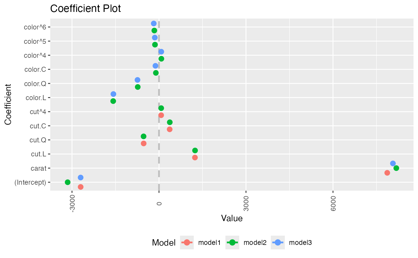
model1 <- lm(price ~ carat + cut, data=diamonds)
model2 <- lm(price ~ carat + cut + color, data=diamonds)
model3 <- lm(price ~ carat + color, data=diamonds)
multiplot(model1, model2, model3)

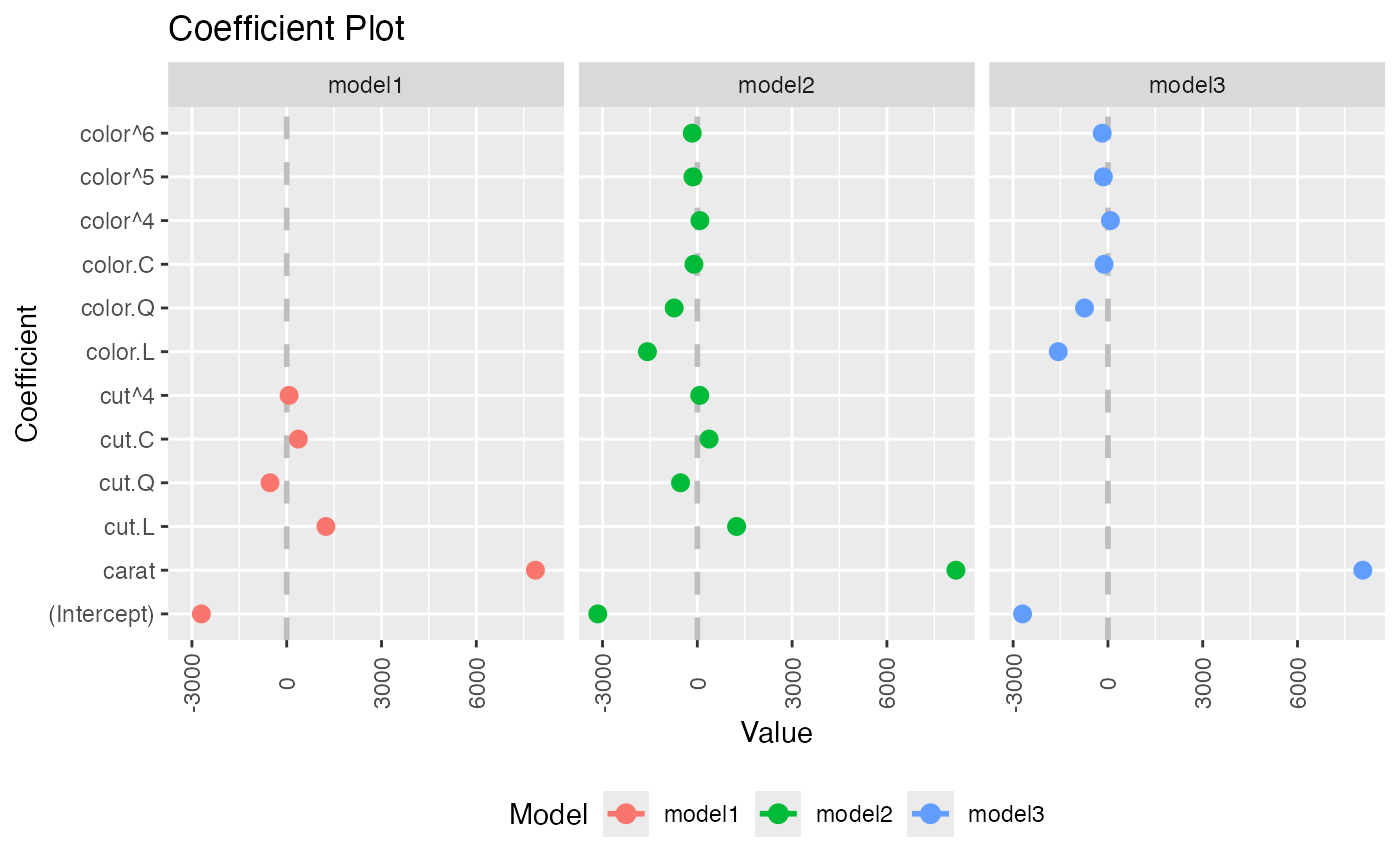
multiplot(model1, model2, model3, single=FALSE)

multiplot(model1, model2, model3, plot=FALSE)
#>          Value Coefficient   HighInner    LowInner   HighOuter    LowOuter
#> 1  -2701.37602 (Intercept) -2685.94495 -2716.80710 -2670.51387 -2732.23818
#> 2   7871.08213       carat  7885.06176  7857.10251  7899.04139  7843.12288
#> 3   1239.80045       cut.L  1265.90049  1213.70040  1292.00054  1187.60036
#> 4   -528.59779       cut.Q  -505.46541  -551.73018  -482.33302  -574.86257
#> 5    367.90995       cut.C   388.12410   347.69579   408.33826   327.48164
#> 6     74.59427       cut^4    90.83386    58.35469   107.07344    42.11510
#> 7  -3149.81846 (Intercept) -3134.06187 -3165.57504 -3118.30528 -3181.33163
#> 8   8183.74295       carat  8197.63996  8169.84595  8211.53696  8155.94894
#> 9   1243.35134       cut.L  1268.08969  1218.61298  1292.82805  1193.87462
#> 10  -531.75088       cut.Q  -509.82486  -553.67689  -487.89885  -575.60291
#> 11   372.05517       cut.C   391.21638   352.89396   410.37759   333.73275
#> 12    76.15453       cut^4    91.54283    60.76622   106.93114    45.37792
#> 13 -1579.17014     color.L -1557.44800 -1600.89228 -1535.72587 -1622.61442
#> 14  -732.84999     color.Q  -712.99047  -752.70952  -693.13094  -772.56905
#> 15  -107.40714     color.C   -88.76901  -126.04527   -70.13088  -144.68339
#> 16    81.63107     color^4    98.74669    64.51546   115.86230    47.39984
#> 17  -138.64340     color^5  -122.46129  -154.82550  -106.27919  -171.00760
#> 18  -161.08789     color^6  -146.40797  -175.76780  -131.72806  -190.44771
#> 19 -2702.23261 (Intercept) -2688.44954 -2716.01569 -2674.66646 -2729.79876
#> 20  8066.62302       carat  8080.66272  8052.58332  8094.70242  8038.54362
#> 21 -1572.19930     color.L -1549.88115 -1594.51745 -1527.56300 -1616.83560
#> 22  -741.14453     color.Q  -720.74595  -761.54312  -700.34736  -781.94170
#> 23  -122.69603     color.C  -103.55099  -141.84107   -84.40594  -160.98612
#> 24    78.76541     color^4    96.34799    61.18283   113.93057    43.60025
#> 25  -144.74008     color^5  -128.11696  -161.36321  -111.49383  -177.98634
#> 26  -180.74716     color^6  -165.66921  -195.82511  -150.59126  -210.90306
#>     Model
#> 1  model1
#> 2  model1
#> 3  model1
#> 4  model1
#> 5  model1
#> 6  model1
#> 7  model2
#> 8  model2
#> 9  model2
#> 10 model2
#> 11 model2
#> 12 model2
#> 13 model2
#> 14 model2
#> 15 model2
#> 16 model2
#> 17 model2
#> 18 model2
#> 19 model3
#> 20 model3
#> 21 model3
#> 22 model3
#> 23 model3
#> 24 model3
#> 25 model3
#> 26 model3
require(reshape2)
#> Loading required package: reshape2
data(tips, package="reshape2")
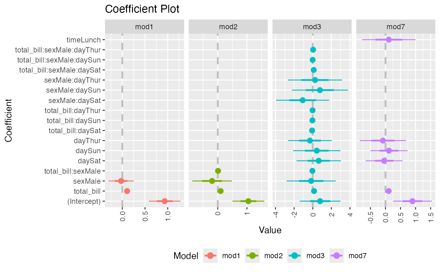
mod1 <- lm(tip ~ total_bill + sex, data=tips)
mod2 <- lm(tip ~ total_bill * sex, data=tips)
mod3 <- lm(tip ~ total_bill * sex * day, data=tips)
mod7 <- lm(tip ~ total_bill + day + time, data=tips)
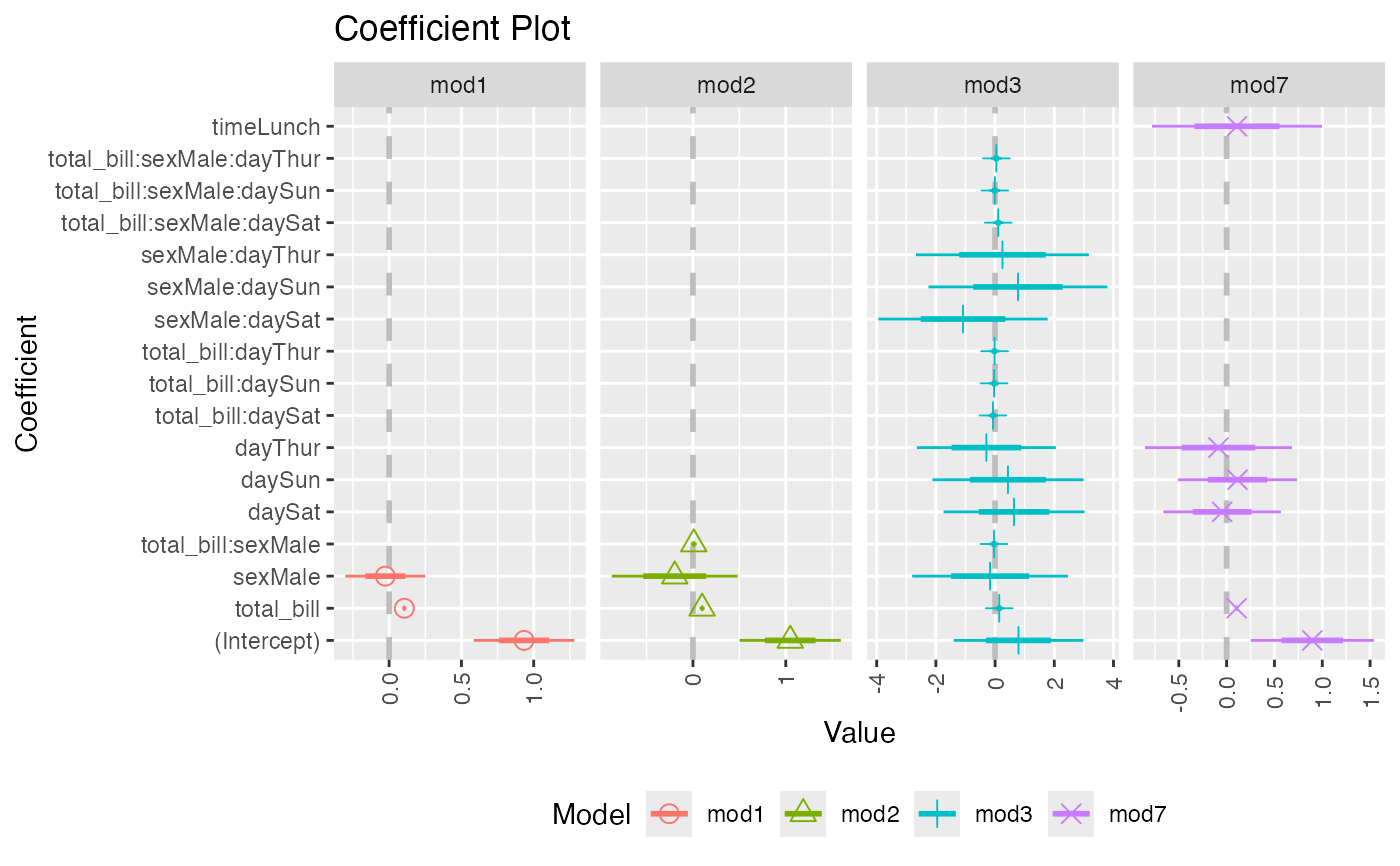
multiplot(mod1, mod2, mod3, mod7, single=FALSE, scales="free_x")

multiplot(mod1, mod2, mod3, mod7, single=FALSE, scales="free_x")

multiplot(mod1, mod2, mod3, mod7, single=FALSE, scales="free_x", plot.shapes=TRUE)

multiplot(mod1, mod2, mod3, mod7, single=TRUE, scales="free_x", 
plot.shapes=TRUE, plot.linetypes=TRUE)

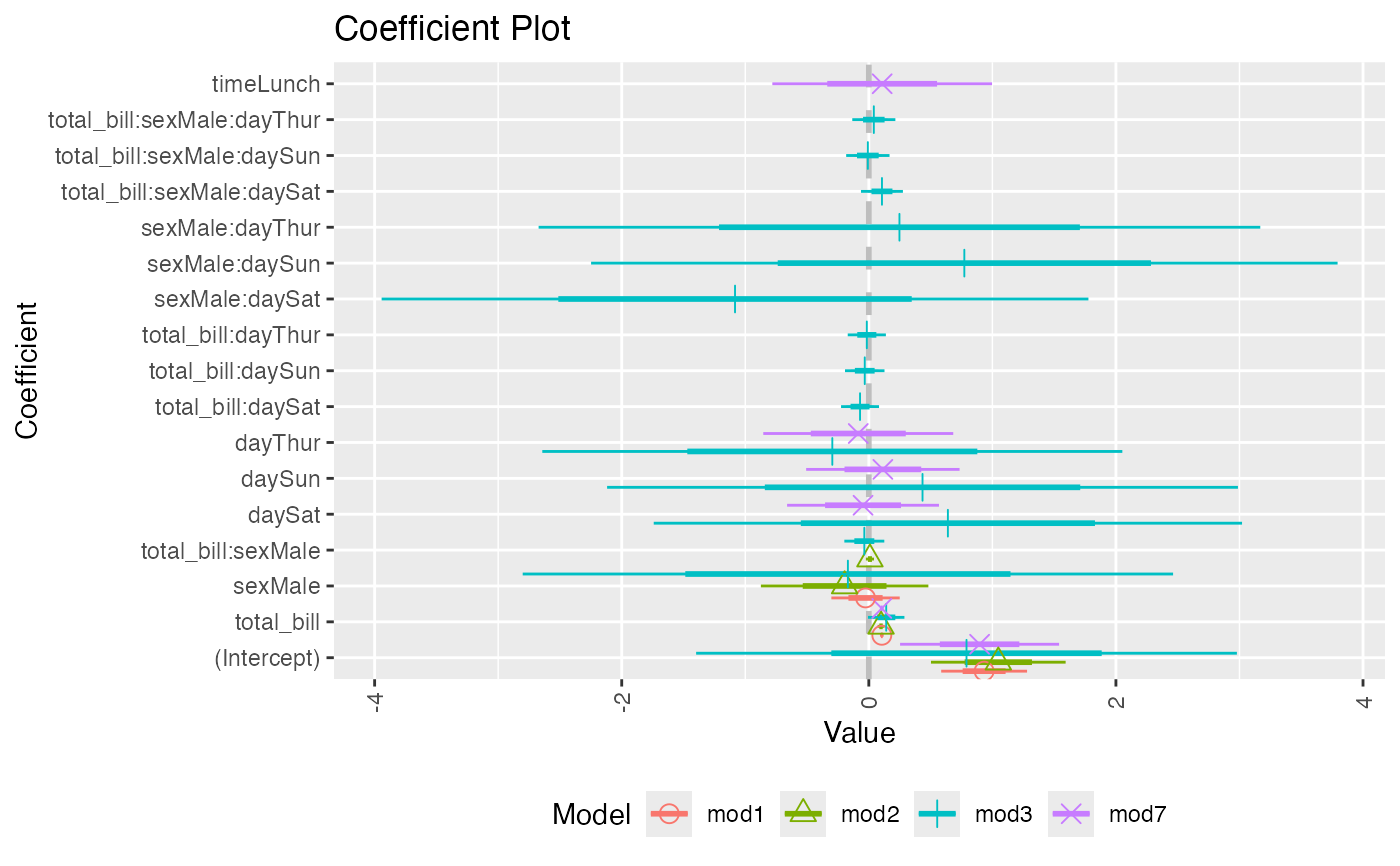
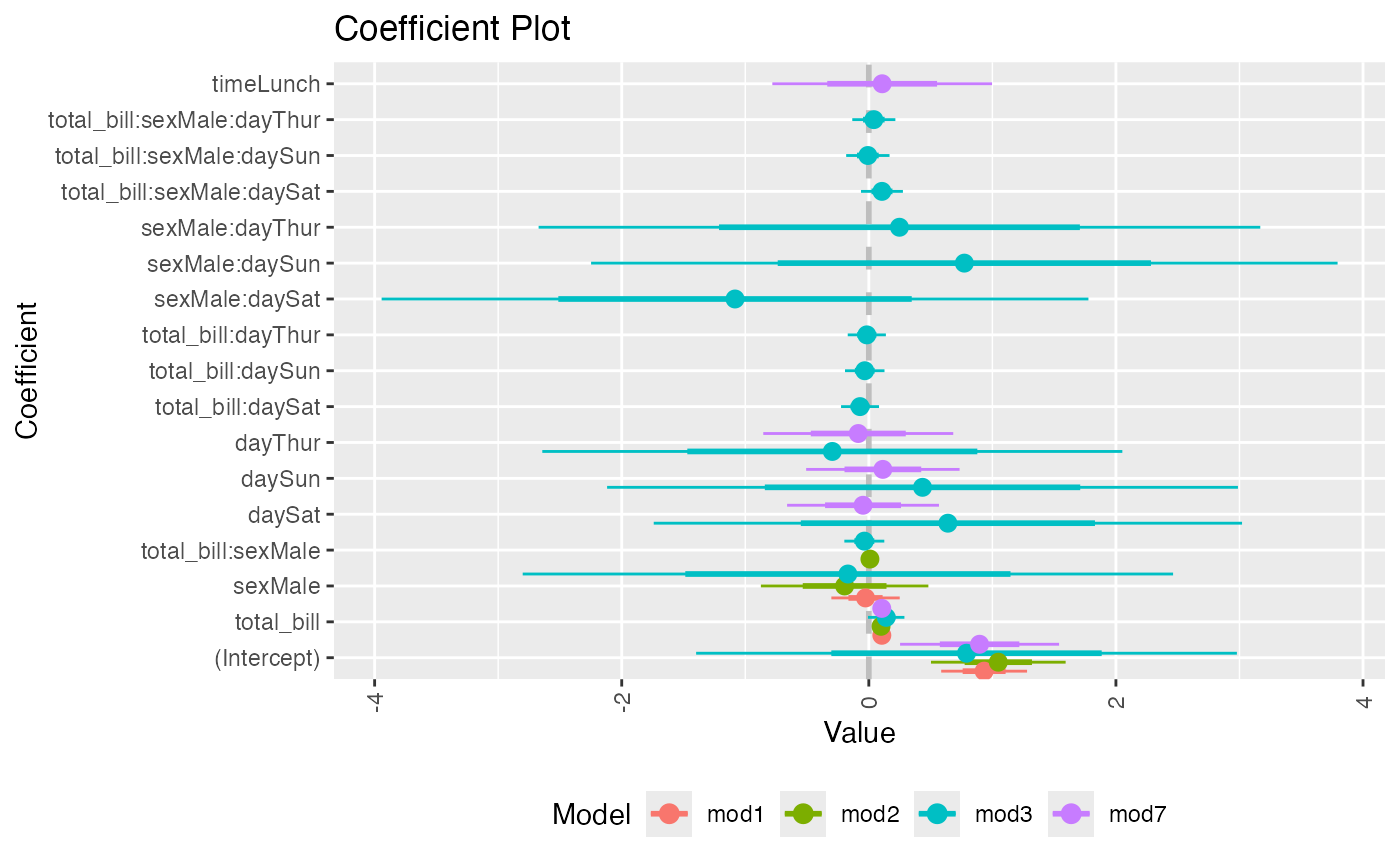
multiplot(mod1, mod2, mod3, mod7, single=TRUE, scales="free_x", 
plot.shapes=FALSE, plot.linetypes=TRUE, legend.position="bottom")

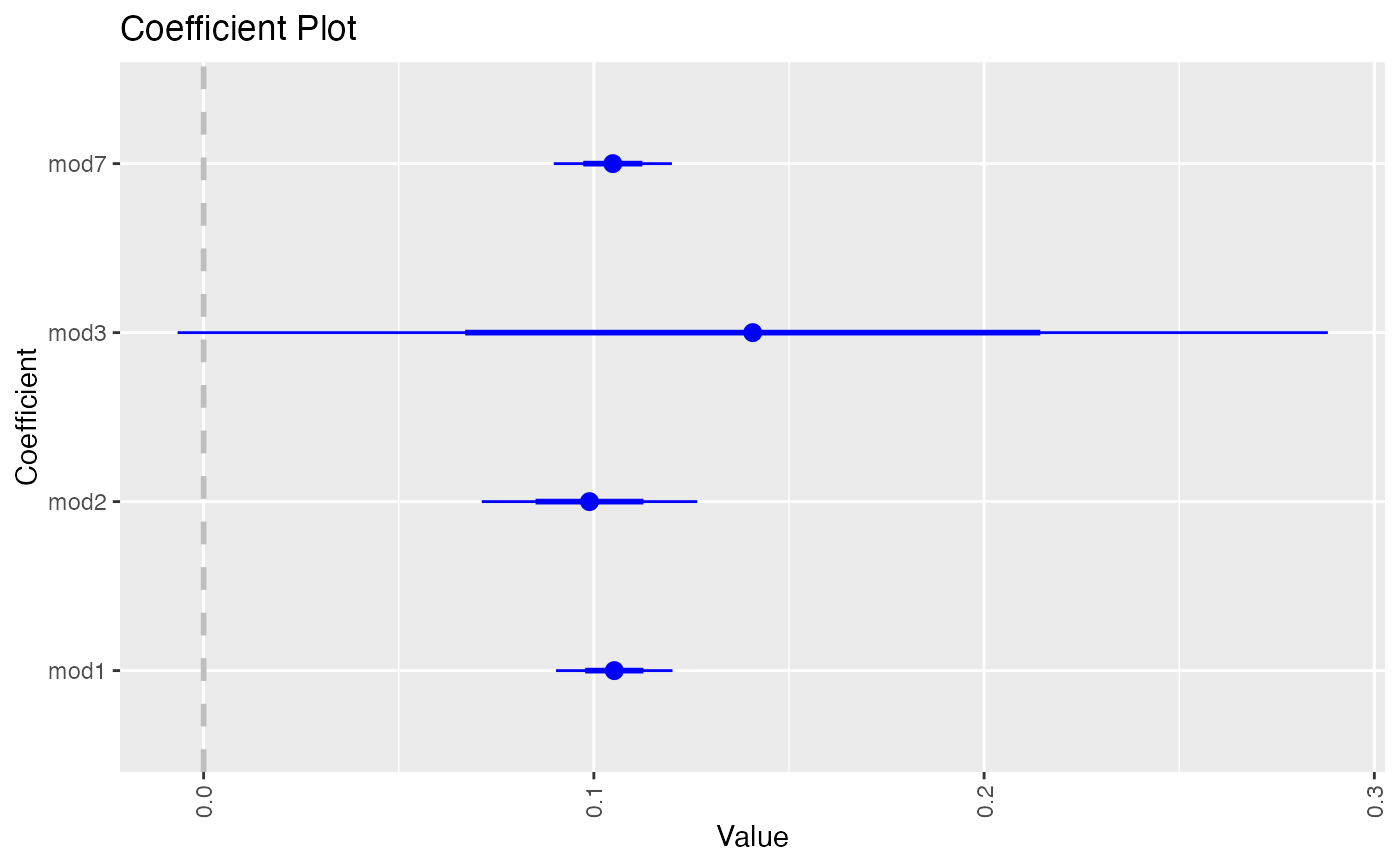
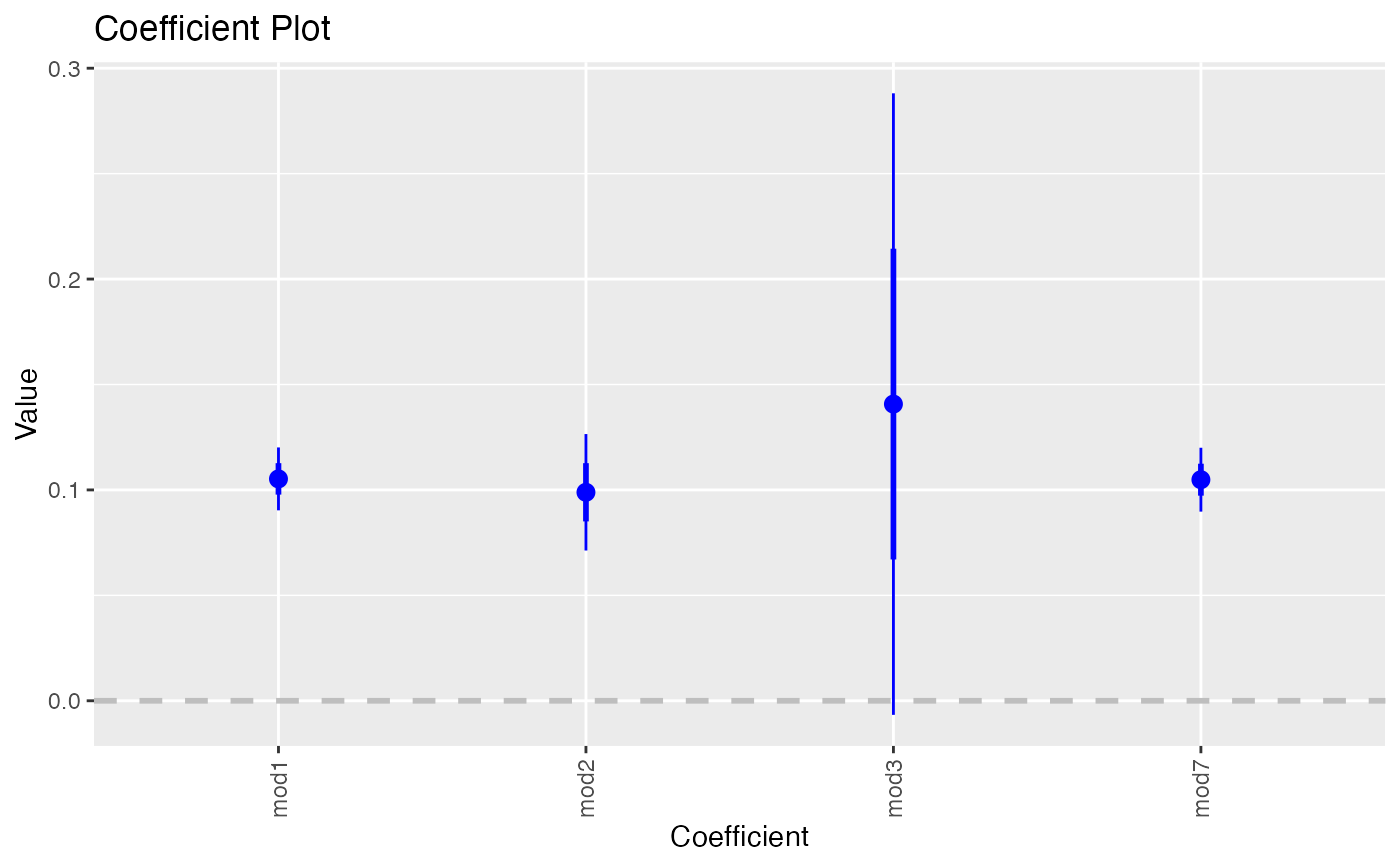
# the secret weapon
multiplot(mod1, mod2, mod3, mod7, coefficients="total_bill", secret.weapon=TRUE)

# horizontal secret weapon
multiplot(mod1, mod2, mod3, mod7, coefficients="total_bill", by="Model", horizontal=FALSE)

Usage

Arguments

Value

Details

See also

Examples